This user case shows the FLUIDAPRO capabilities concerning water hammer analysis in a pipe using a fluid with real properties (two phase flow). The pipe is simulated by the Pipe component, which takes into account inertia forces, pressure losses and phase changes.
This pipe is connected to two boundary conditions (inlet and outlet components) by the resistive components “junction” and “Jun_TMD”. This last component allows the user to impose a value for the mass flow along the system. In this case, the component AnalogSource from the CONTROL library is used to establish this value.
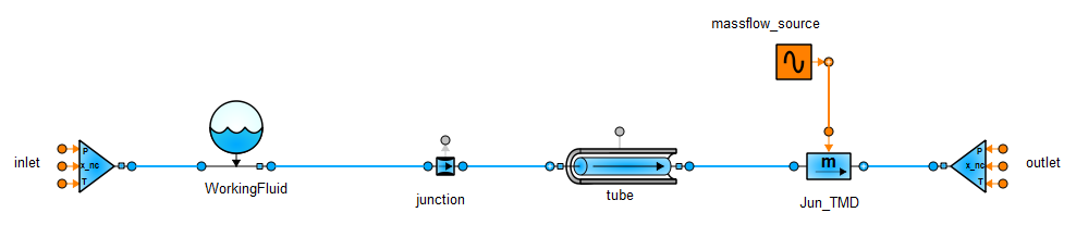
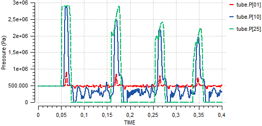
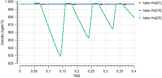
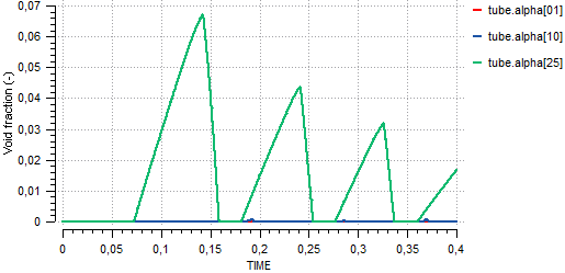
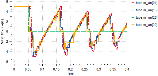
An initial steady state is reached to determine the pipe conditions at a constant mass flow. A transient evolution is started by a sudden flow reduction on the right side. The plots below show the evolution of pressure, density, void fraction and mass flow inside the pipe during the water hammer. The following phenomena can be seen:
- Pressure rises (pcv) are due to the wave trips caused by a sudden stop of the fluid. This wave is reflected in the open end as a negative flow.
- When this backflow is stopped again at the closed end, the “negative” pressures that should be created are limited to the vapour pressure.
- The corresponding vapour bubble formation then takes place. This causes a water column separation, and the column enters the tank.
- Bubble collapse begins when this liquid column is stopped by the tank pressure and begins to enter the pipe causing the vapour to collapse.
- A new cycle starts when the liquid column is stopped at the closed end when the vapour is eliminated.
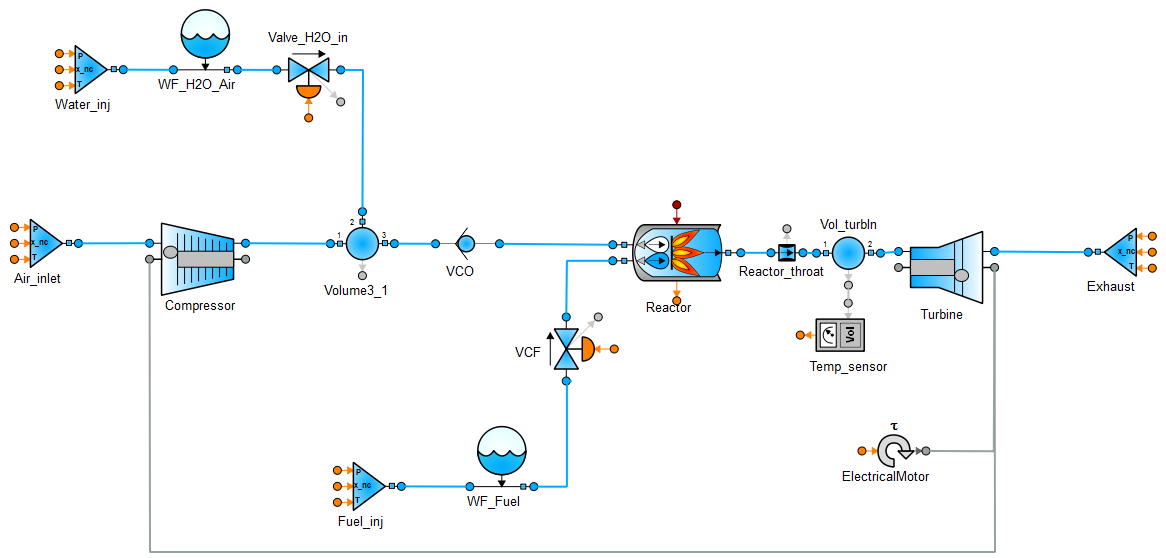
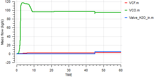
This model represents a simplified gas turbine for industrial applications. The air is taken from the atmosphere, compressed and then mixed with a small quantity of water. The mixture enters in a reactor together with fuel, which provokes the burning. The gases produced in the combustion move a turbine placed downstream from the reactor, which extracts energy for an electrical motor and also to move the compressor.
The injection of water and fuel can be regulated, depending on the target working point, by opening or closing the corresponding valve. The power extracted can also be set in the electrical motor.
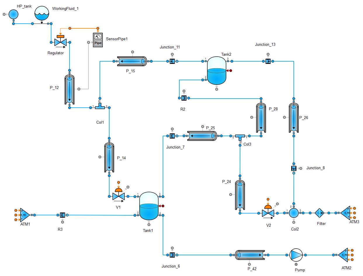
The following schematic has been built for this example:
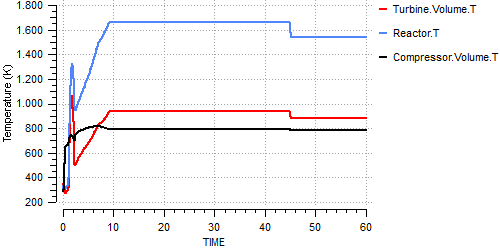
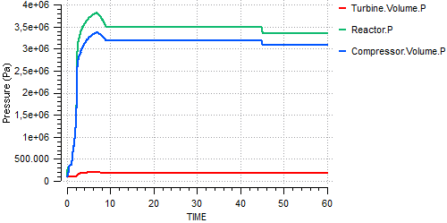
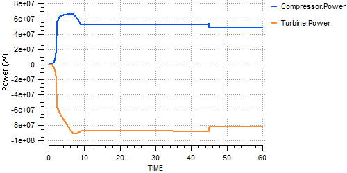
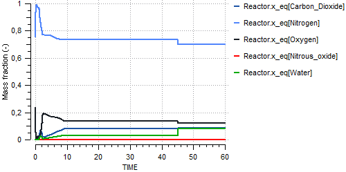
The following plots show the evolution of temperatures, pressures and mass flows in different points of the system, the power in the turbo-machinery and the mass fraction of chemicals present in higher percentage in the reactor:
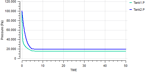
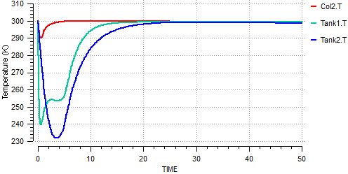
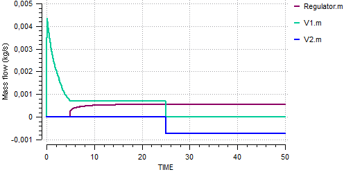
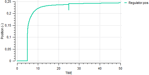
The model represents a system that deals with the extraction of polluted air from several places where high cleanliness conditions are required (“Tank1” and “Tank2). Low vacuum is achieved by means of a water-ring pump. The pressure-regulator keeps the vacuum-level at a certain value. It is a valve with variable throat section driven by the upstream/downstream pressure difference according to opening/closing settings.
The circuit contains a porous filter. The pressure loss in this component is calculated as a linear relation between flow and pressure-drop for given reference conditions. Two on-off valves (“V1” and “V2”) control the incoming atmospheric air, either from the pressure regulator branch or the filter branch. Additionally, there are two calibrated holes “R2” and “R3” (quadratic restrictors). Some other elements are used to connect all the parts of the circuit, such as pipes, junctions, and tee joints.
Finally, the environmental conditions such as ambient pressure and temperature are simulated using constant pressure tanks (“HP_tank”, “Ambient1”, “Ambient2”, and “Pump_exit”) and thermal boundary nodes (“Wall_BT1” and “Wall_BT2”).
At the beginning of the simulation, valve “V1” is opened and “V2” is closed, permitting a direct air flow from the external atmosphere “HP_tank” to “Tank1”. In this first stage, the air in the low pressure area is pumped out reaching the desired pressure conditions in “Tank1” in less than 5 seconds. The pressure drops until the pressure difference in the regulator is enough to open it. After this, the pump maintains the pressure level in the tanks by pumping out the incoming air flow from the regulator, filter branches and tank leaks.
The valves are kept in their initial status for up to 25 seconds, at which point “V1” is closed and “V2” is opened. The air coming from the pressure regulator then reaches “Tank1” after passing through “Tank2”. The change of valve status can be clearly seen in the mass flow plots. The pressure level of the tanks is kept in the same way, as in the previous stage. Finally, the simulation is stopped at 100 seconds.
The following plots illustrate pressure and temperature evolution in the tanks, mass flow through the valves and the regulation position of the pressure regulator.
In this user case, some FLUIDAPRO components are arranged to simulate the behaviour of an actuator commanded by a signal applied to a 4-way valve (component “Ev_4w”). Depending on the working fluid selected, this model represents a hydraulic or pneumatic actuator (component “Actuator_2C”).
The actuator contains two chambers separated by a piston. This piston moves according to the chamber pressures, the spring and Coulomb friction forces, and the external forces. The 4-way valve connects the actuator chambers to the low and high-pressure tanks. When the valve has no signal, actuator “Volume1” is set to atmospheric conditions and actuator “Volume2” is connected to the high-pressure tank. These connections are reversed when a signal is applied to the valve. Other elements are used to connect all the parts of the circuit, such as pipes and junctions. The diameter considered in all these items is 0.006 metres.
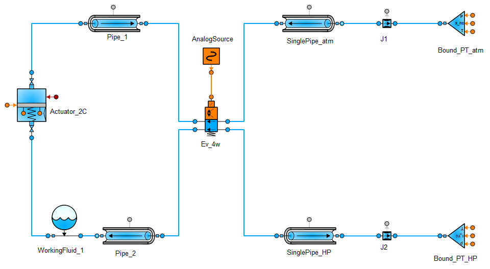
The mass of the piston is 6.4 kg, its effective area on its two sides is 0.001963 m2 and the length of stroke is 0.051 metres. Chamber dead volumes are 6.1 • 10-5 m3 and 2.5 • 10-5 m3 for “Volume1” and “Volume2”, respectively. The equivalent throat diameters (0.96 mm) depend on the direction of flow (different coefficients for direct and reverse pressure losses). The effective EV throat diameter of the valve is 0.00357 metres.
In this model, the spring and Coulomb friction data are set to zero, but the following specific equations are written in the continuous block of the model defining the piston-chamber interaction as shown in the figure below:
Spring force = 0.5 • (fic1 + fic2 / (rpiston • cos(ø))
Coulomb force = 0.5 • (fic1 – fic2) * tanh(1000 • vpiston) / (rpiston • cos(ø))
The use of the hyperbolic tangent gives zero Coulomb forces at zero speed. “fic1” and “fic2” are the interpolation results in the data tables of measured torque (at positive speed “f1_theta” and negative speed “f2_theta”):
fic1 = linearInterp1D(f1_theta, ø)
fic2 = linearInterp1D(f2_theta, ø)
ø = ø1 + asin(xpiston + x0) / rpiston
x0 = rpiston • sin(ø1);
Finally, the environmental conditions are set by the components “Bound_PT_atm” and “Bound_PT_HP”. The pressure is set to 0.1 MPa and 7.0 MPa, respectively. Additionally, the temperature is set to 300K in both elements.
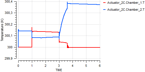
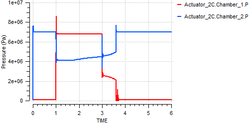
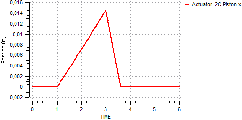
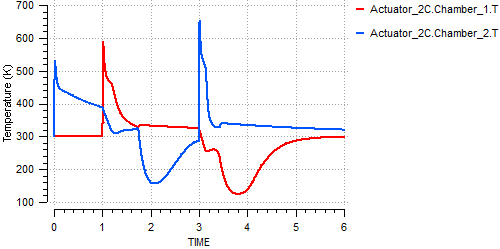
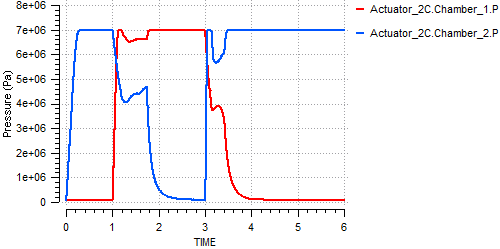
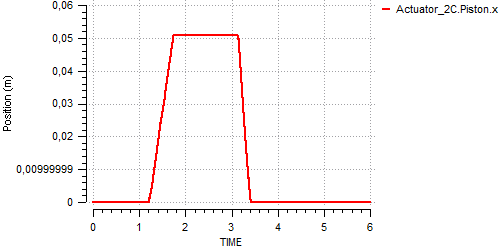
In the first stage of the simulation, the 4-way valve signal is set to 0. That means that chamber 1 of the actuator is set to atmospheric conditions and chamber 2 is connected to the high-pressure tank. After a brief stabilisation period of less than 0.25 seconds, this chamber reaches high-pressure conditions. The piston remains motionless throughout the process.
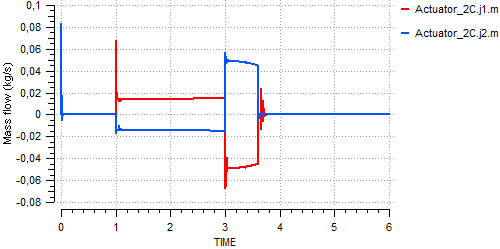
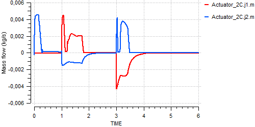
After 1 second, the flow paths of the chambers are reversed when the valve signal changes to 1. Then the pressure in chamber 1 starts growing while the pressure in chamber 2 drops. Soon after the pressure in both chambers crosses, the piston starts moving once the pressure difference is enough to overcome the friction forces. Pressure oscillation can be seen in both chambers while the piston is moving. This oscillation disappears when the piston reaches its end stop.
In the last part of the simulation, a 0 signal is again applied to the valve after 3 seconds, the pressure in the chambers is then reversed and the piston moves backwards. As in the previous phase, some pressure oscillatory phenomena are also seen, but they are different because of the faster movement of the piston. The different orifice area in each chamber causes this asymmetry. Finally, the simulation stops after 6 seconds.
The following plots illustrate the actuator behaviour using Helium gas as the working fluid: Actuator piston position, pressure evolution in the actuator chambers, temperature evolution in tank walls, and actuator chamber incoming mass flow.
The following plots illustrate the actuator behaviour using liquid water as the working fluid: Actuator piston position, pressure evolution in the actuator chamber, and actuator chambers incoming mass flow. The movement is slower because of the greater orifice resistance (pressure drop) with water for the same orifice area.